Introduction
Owing to the seemingly counter-intuitive effects of quantum superposition and entanglement, a quantum computer has the potential to perform certain calculations that would otherwise be impossible on a regular device. The possibilities, ranging from prime factorisation [1] to modelling of quantum systems [2], seem endless. Building one, however, is a rather tricky endeavour. The DiVincenzo [3] criteria outline the required conditions to construct a working and scalable quantum computer. Arguably the most critical of which is the need for a system to effectively be isolated from the rest of the universe so as not to be a victim of decoherence, which destroys quantum information.
Experimentalists are working on creating coherent systems consisting of components such as cold neutral atoms [4], photons [5], and ions [6]. In the developmental meantime, we can theoretically model such systems of qubits to explore how we can limit decoherence.
A classically ergodic system is considered thermalised if it has been allowed to explore its entire phase space for a sufficiently long time. Once thermalised, it will have an equal chance of being in any microstate. This system is described by the famous microcanonical ensemble [7].
Unlike classical systems, where ergodicity and thermalisation are well understood, quantum systems are much more elusive. The eigenstate thermalisation hypothesis was proposed in an attempt to explain when and why a quantum system thermalises to a classical microcanonical ensemble [8]. Consider a finite isolated system which has eigenstates and eigenenergies which can be measured using observables. The operator will have expectation values  but we can also write them in terms of their microcanonical average and variance
  [9]. The hypothesis states that the fluctuations of the expectation values between different eigenstates will be so small that we can evaluate the thermal ensemble from one eigenstate [10].
It was previously understood that the only way to break this hypothesis was if there was a set of  independent conserved quantities [11,12] in the system, where is the number of degrees of freedom. However, a new Hamiltonian has been discovered [13] which breaks this hypothesis. So far, no set of so many quantities have been found. The experiment involved a one-dimensional array of atoms which could each be individually prepared in either their ground or highly excited Rydberg state [14]. In most preparations of the initial state, the system thermalised and became chaotic. However, certain prepared states appeared to remain coherent for longer than expected.
In an attempt to explain how this occurs we must look to quantum scars which are phenomena that arise in quantum chaos theory [15]. An example [16,17] of this effect consists of a system comprising of a single particle in a stadium. Classically, [18] the path the particle will take is chaotic with a set of unstable periodic orbits. At the quantum level, the eigenstate amplitudes surrounding these orbits are enhanced. A recent article [19] demonstrates potential evidence for the discovery of the many-body analogue of this effect in the experiment described above. The authors also proclaim that the system demonstrates weak ergodicity breaking meaning that whether the system explores all possible states depends strongly on its initial configuration.
The following sections will explore whether quantum scars are responsible for the observed weak ergodicity breaking, investigate other potential explanations [19,20,21,22] and introduce the interaction distance [24,25] as a potential tool to further examine the origins of this notable phenomenon.
Rydberg Chain
The time evolution of any quantum system can be reduced to defining an initial configuration and a Hamiltonian by simply integrating the Schrödinger equation to evaluate a time evolution operator. For the case that the Hamiltonian does not depend on time its time evolution is described by
(1) 
In practice, this is generally not so easy to evaluate since to find the exponential of a matrix it is first necessary to find its eigenvalues and eigenvectors. If we have a system of size N composed of individual components of size M, then the total dimension of the system is  . Thus, the computational complexity to exponentiate the matrix is of order
  . As suggested by Feynman in 1981 [2], rather than evaluating such complicated calculations, we could instead build a simulator which naturally evolves in time and exploits the quantum effect of superposition.
It is now experimentally possible to realise previously theoretical [28] Hamiltonians consisting of single atoms [29]. By directing a laser onto a cold neutral atom, experimentalists [4,30] have been able to induce sinusoidal Rabi oscillations [31] in the amplitude of their ground and excited state. By adjusting the Rabi frequency,  , and detuning,
  , it is possible to manipulate and control these oscillations.
The experiment [13] that inspired the investigation of many-body scars consisted of a linear array of \ce{^{87}Rb} atoms with the Hamiltonian
(2) 
where the first two terms simply correspond to the summation of the atom-light interaction Hamiltonian. The Pauli matrix  flips a state between its excited and ground state. In the experiment a secondary beam, contained within the existing and , was introduced to reach the highly excited Rydberg states [32]. These states are highly repulsive when next to each other and thus contribute to the final interaction term. By first using optical pumping to initialise the ground state, the group then varied the detuning to prepare a
  product state consisting of alternating excitations.
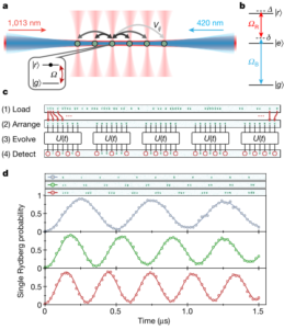
Experimental realisation of the Rydberg chain as printed in [12]. a) shows the arrangement of the atoms in a one-dimensional optical lattice. b) there are two driving lasers, one to excite the atom to its excited state  and another to drive it to its even more highly excited Rydberg state
  . The Rydberg excitations are highly repulsive of each other if they are sufficiently close. c) demonstrates an example of the experimental protocol in which atoms are programmed by loading and arranging them into the required states. After allowing the system to evolve in time their state is recorded. d) shows that by arranging atoms far enough away from each other we see regular Rabi oscillations. If they are then arranged into blocks of two or three atoms there can only be one excitation per block. This corresponds to an enhanced Rabi frequency.
Theoretical Model
To investigate the origin of these oscillations and to explain this apparent weak ergodicity breaking, the Hamiltonian is first simplified. By introducing the projection operator,  , we can break the Hilbert space into separate components, effectively restricting the accessible states to those which do not contain neighbouring excitations. In the limit where
  and
and  the simplified Hamiltonian becomes [36]
(3) 
For further simplicity we consider periodic boundary conditions, meaning that  is equivalent to
  .
.
The reduced Hilbert space for this Hamiltonian consists only of the states which do not contain adjacent excited atoms. The dimension of which is equal to  [22] where the term
  is the
  Fibonacci number. This is a great reduction from the previous
  basis states, as can be seen in the following figure.
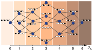
A visual demonstration of the reduced Hilbert space as printed in [17]. The allowed states are grouped by their Hamming distance,  , which gives the fewest number of spin flips required to get back to the
  product state.
 . In order to increase the limit of the system size symmetries are employed. In this example, translational symmetry is identified but this can be further extended using particle-hole and spatial inversion symmetry [22].
By its definition the translation operator acts on a state as
(4) 
and thus we can identify that  .
.
Utilising this fact and following the method of [37] we identify a set of momentum states with eigenvalues  which are valid for the following momenta
(5) 
Any momentum state  can be assembled via a basis state
  and its translations
(6) 
where  is the periodicity of the basis state.
Since  the Hamiltonian will be block diagonal in the basis of the eigenstates of
  . To see this we evaluate the action of the Hamiltonian on an arbitrary momentum state as
(7) 
The output of the Hamiltonian parts  on a reference state will also be related to a reference state within some
  number of translations. We are able to extract matrix elements of the form
(8) 
which gives a set of matrices corresponding to each allowed momentum, further increasing the size of systems we can feasibly model on a classical computer. The article [25] demonstrates a simulation of size  using the infinite time evolving block decimation method [38]. This only gives results valid to time
  but this is enough to demonstrate the oscillations observed in the experiment. The following figure shows the fidelity of the time evolution of the initial state
  . In the momentum basis this is
  . An example of the entanglement entropy for
  starting in the state is plotted in the figure below.
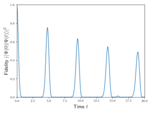
Overlap of the initial state prepared in the state with its evolved state at time  for a system of
  sites. Exact diagonalisation was used to find the eigenenergies and eigenstates utilising translational symmetry with periodic boundary conditions. Unusually coherent oscillations of the overlap are clearly visible.
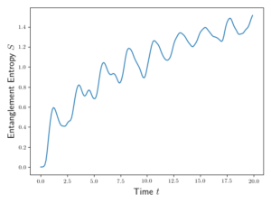
The initial state is prepared in the state and allowed to evolve in time for a system of sites. The entanglement entropy  is calculated at each point. We are limited to a size of because Schmidt decomposition [40] has yet to be implemented to speed up the entropy calculation.
The Hamiltonian was first constructed for in the product state basis. The eigenenergies and eigenstates were found and then overlapped with the state.  special states emerge which have particularly high overlap with the periodic state.
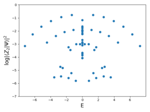
In an attempt to explain these long-lasting oscillations, the article [19] demonstrates an unusually high overlap between eigenstates and so-called special states. The energy separation between these special states matches the frequency of oscillations of the entanglement entropy. A plot of these states can be seen in the above figure.
The article then goes further by demonstrating that it is possible to approximate these special states using a forward scattering approximation by splitting the Hamiltonian into operators 
(9) 
where  and
and  . These operators have the effect of increasing or decreasing the Hamming distance [40], which gives the number of spins required to flip to reach some initial state.
We obtain a non-interacting Hamiltonian of the form
(10) 
with the tridiagonal terms
(11) 
This free model is reported to have errors less than  for a chain of .
The authors propose that this demonstrates a new universality class of quantum dynamics and suggest that this motivates further research into this class of dynamics. To enhance this argument, the paper considers a potential alternative. They make the claim that no proximate integrable system could be responsible for the non-ergodic dynamics because the level statistics [35] approaches the Wigner-Dyson distribution as the system size is increased. This is in opposition to a trend towards a Poisson distribution which would be expected for integrable systems. It is noted that the “Golden chain” system [41], which is integrable, is qualitatively similar to the Rydberg chain. The authors argue that, despite this, the two Hamiltonians differ too much to be considered a weak deformation of each other.
Since the publication of this article there have been further theoretical explorations of the experiment. Reference [21] demonstrates that a deformation of the Hamiltonian can enhance both coherence of the oscillations and proximity to integrability based on its level statistics. They do not demonstrate what the parent Hamiltonian is nor do they explain the importance of the distinction between a subclass of integrability and an entirely new class.
Reference [47] introduces a manifold of only locally entangled spin states and derives their equations of motion using matrix product states and the time-dependent variational principle [42]. The equations of motion of the product state only explores a special low-entanglement manifold of the Hilbert space. This is like the single particle case of quantum scars in which the classical unstable orbits are enhanced.
Further exploration [19] by the authors of the original theory paper counters the proximate integrability argument by demonstrating that the quantum scars appear to be stable under various perturbations. Specifically, it is shown that there is a strong correlation between perturbations near the forward scattering approximation and the robustness of quantum scars.
Interaction Distance
Free fermion systems are surprisingly sprawling across physics given their simplicity to solve. It is possible to directly diagonalise their system Hamiltonian by constructing a new set of eigenmodes. This allows them to be solved as a set of independent and uncorrelated single particle modes. The energy spectrum of such a system is given by [24]
(12) 
where  represents the energies of the eigenmodes and the value from the number operator,
  , can be
  or
or  . When considering more complicated interacting systems it would clearly be useful to instead express it as a free fermion system or alternatively find one that is very close.
Reference [25] demonstrates a new tool, the interaction distance, for efficiently calculating the proximity of any given interacting fermion system to its closest free system by calculating its entanglement spectrum [43]. In addition, it outlines a method for extracting the composition of the stated nearby free system.
A system in thermal equilibrium can be represented by the density matrix [7]
(13) 
where  is the inverse thermodynamic temperature and
  is the partition function normalised over all temperatures. A free system can be accurately described by Equation (13) and its eigenvalues are given with respect to the eigenvalues of the energy
  of the system.
If we instead have an interacting system, we can construct a reduced density matrix from an arbitrary eigenstate  of its Hamiltonian. This reduced density matrix is given by the partial trace [44] over the entire density matrix of the state
(14) 
The goal is to identify the distance between this arbitrary density matrix and some free density matrix. To find this distance, we require a manifold  of all the free fermion states which are of the form
(15) 
The interaction distance is thus defined as a minimisation
(16) 
where the quantity  is the trace distance [44].
The authors demonstrate its utility with the one-dimensional Ising model
(17) 
with  and
and  representing the ferromagnetic and antiferromagnetic systems respectively.
The quantum critical point in the ferromagnetic Ising model occurs at  . This is visible in the interaction distance phase diagram which shows a relatively high interaction distance surrounding the critical point. More interestingly a critical line emerges in the antiferromagnetic system spanning through the classical critical point
  , where the spins can be treated as classical objects [45]. As the system size is increased the interaction distance of the regions surrounding criticality decrease whilst those on the critical line remain constant.
The Rydberg blockaded system has interacting terms and thus it would be interesting to explore the phase diagram surrounding the Hamiltonian with some perturbations. It may demonstrate that it has closest proximity to the free Hamiltonian of Equation (10), further supporting the quantum scar case, or else in unexpected regions.
Conclusion
This review has introduced both the concept and importance of quantum many-body scars as realised in the experiment [13] with the Rydberg blockade chain Hamiltonian and explored in [25]. A demonstration of the analytical realisation of the reduced Hilbert space has been presented. A computation of the eigenstates using diagonal symmetries has also been used to plot the time evolution for the product state.
A critical analysis of the validity of the suggestion and counterargument of a new universality class was also discussed. The concept of the many-body scarred states is strongly supported by other work [23,47] although whether there exists a parent proximate Hamiltonian is still disputed.
A novel tool to analyse the phase space of the Hamiltonian has also been considered, along with an example of an exploration of a similar interacting fermion system as described in [25]. This is a relevant source of research to be further explored for this project. The code to calculate the interaction distance and the closest free system to an arbitrary system is available online. The input required is simply the entanglement spectrum. The evaluation of the entanglement spectrum for the special states will be the next step in this project. By evaluating the interaction distance of these states using the code it may be possible to identify behaviours of the Rydberg system in the thermodynamic limit.
Finally, in this project, I hope to be able to develop and define some form of \textit{integrability distance}. This would allow an exploration of whether there exists some proximate Hamiltonian and a measure of its closeness to the Rydberg chain Hamiltonian (2). A stronger understanding of the theory of integrability, the interaction distance and the Bethe ansatz [48] will be required in order to develop this idea further. Such a metric could also give means to explore alternative Hamiltonians with scarred states that could lead to realisable demonstrations of weak ergodicity breaking. New such Hamiltonians could lead to a greater understanding of the eigenstate thermalisation hypothesis and potentially lead to new methods to develop quantum devices with longer lasting coherence.
References
[1] Shor, P. W. (1995). Polynomial-Time Algorithms for Prime Factorization and Discrete Logarithms on a Quantum Computer. SIAM Review, 41(2), 303–332.
[2] Feynman, R. P. (1982). Simulating physics with computers. International Journal of Theoretical Physics, 21(6–7), 467–488. http://infoscience.epfl.ch/record/1143
[3] DiVincenzo, D.P. (2000), The Physical Implementation of Quantum Computation. Fortschr. Phys., 48: 771-783.
[4] Walker, T. G., & Saffman, M. (2012). Entanglement of Two Atoms Using Rydberg Blockade. Advances in Atomic, Molecular and Optical Physics, 61(January), 81–115.
[5] Politi, A., Matthews, J. C. F., Brien, J. L. O., Politi, A., Matthews, J. C. F., & Brienf, J. L. O. (2009). Shor’s Quantum Factoring Algorithm on a Photonic Chip. Science, 325(5945), 1221.
[6] Blatt, R., & Wineland, D. (2008). Entangled states of trapped atomic ions. Nature, 453(7198), 1008–1015.
[7] Plischke, Michael., & Bergersen, Birger. (2006). Equilibrium statistical physics. World Scientific.
[8] Rigol, M., Dunjko, V., & Olshanii, M. (2008). Thermalization and its mechanism for generic isolated quantum systems. Nature, 452(7189), 854–858. http://dx.doi.org/10.1038/nature06838
[9] Srednicki, M. (1994). Chaos and quantum thermalization. Physical Review E, 20(2), 888–901.
[10] Deutsch, J. M. (2018). Eigenstate thermalization hypothesis. Reports on Progress in Physics, 81(8).
[11] M. Gaudin and J.-S. Caux, The Bethe Wavefunction (Cambridge University Press, 2014).
[12] D. A. Huse, R. Nandkishore, V. Oganesyan, A. Pal, and S. L. Sondhi, Physical Review B – Condensed Matter and Materials Physics 88, 1 (2013).
[13] H. Bernien, S. Schwartz, A. Keesling, H. Levine, A. Omran, H. Pichler, S. Choi, A. S. Zibrov, M. Endres, M. Greiner, V. Vuletic, and M. D. Lukin, Nature 551, 579 (2017).
[14] D. Jaksch, J. I. Cirac, P. Zoller, S. L. Rolston, R. Côté, and M. D. Lukin, Physical Review Letters 85, 2208 (2000).
[15] Z. Rudnick, Notices Amer. Math. Soc. 55, 32 (2008).
[16] E. J. Heller, Physical Review Letters 53, 1515 (1984).
[17] S. W. McDonald and A. N. Kaufman, Physical Review Letters 42, 1189 (1979).
[18] G. Benettin and J. M. Strelcyn, Physical Review A 17, 773 (1978).
[19] C. J. Turner, A. A. Michailidis, D. A. Abanin, M. Serbyn, and Z. Papić, Nature Physics 14, 745 (2018).
[20] W. W. Ho, S. Choi, H. Pichler, and M. D. Lukin, ArXiv e-print (2018), arXiv:1807.01815v1.
[21] V. Khemani, C. R. Laumann, and A. Chandran, ArXiv e-print (2018), arXiv:1807.02108.
[22] C. J. Turner, A. A. Michailidis, D. A. Abanin, M. Serbyn, and Z. Papić, Physical Review B – Condensed Matter and Materials Physics 98, 155134 (2018).
[23] C.-J. Lin and O. I. Motrunich, ArXiv e-print (2018), arXiv:1810.00888.
[24] J. K. Pachos and Z. Papi, SciPost Phys. Lect. Notes 4 (2018).
[25] C. J. Turner, K. Meichanetzidis, Z. Papić, and J. K. Pachos, Nature Communications 8 (2017).
[26] J. J. Sakurai and S. F. Tuan, Modern quantum mechanics (Benjamin/Cummings, 1985).
[27] G. H. Golub and C. F. Van Loan, Matrix Computations, 3rd ed. (The John Hopkins University Press, 1996).
[28] G. K. Brennen, C. M. Caves, P. S. Jessen, and I. H. Deutsch, Physical Review Letters 82, 1060 (1999).
[29] T. A. Johnson, E. Urban, T. Henage, L. Isenhower, D. D. Yavuz, T. G. Walker, and M. Saffman, Physical Review Letters 100, 2 (2008).
[30] L. Isenhower, E. Urban, X. L. Zhang, A. T. Gill,
T. Henage, T. A. Johnson, T. G. Walker, and
M. Saffman, Physical Review Letters 104, 8 (2010).
[31] R. Loudon, The quantum theory of light (Oxford University Press, 2000).
[32] B. Sun and F. Robicheaux, New Journal of Physics 10, 045032 (2008).
[33] W. Happer, Reviews of Modern Physics 44, 169 (1972).
[34] R. Nandkishore and D. A. Huse, Annu. Rev. Condens. Matter Phys. 6, 15 (2015).
[35] L. D’Alessio, Y. Kafri, A. Polkovnikov, and M. Rigol, Advances in Physics 65, 239 (2016).
[36] I. Lesanovsky, Physical Review Letters 106, 1 (2011).
[37] A. W. Sandvik, AIP Conference Proceedings 1297, 135 (2010).
[38] J. Jordan, R. Orús, G. Vidal, F. Verstraete, and J. I. Cirac, Physical Review Letters 101, 8 (2008).
[39] A. Pathak, Elements of quantum computation and quantum communication (CRC Press, 2013).
[40] D. J. C. MacKay, Information theory, inference, and learning algorithms (Cambridge University Press, 2003).
[41] A. Feiguin, S. Trebst, A. W. Ludwig, M. Troyer, A. Kitaev, Z. Wang, and M. H. Freedman, Physical Review Letters 98, 1 (2007).
[42] J. Haegeman, J. I. Cirac, T. J. Osborne, I. Pižorn, H. Verschelde, and F. Verstraete, Physical Review Letters 107, 1 (2011).
[43] H. Li and F. D. M. Haldane, Physical Review Letters 101, 1 (2008).
[44] M. A. Nielsen and I. L. Chuang, Quantum Computation and Quantum Information (Cambridge University Press, Cambridge, 2010).
[45] A. A. Ovchinnikov, D. V. Dmitriev, V. Y. Krivnov, and V. O. Cheranovskii, Physical Review B – Condensed Matter and Materials Physics 68, 1 (2003).
[46] F. Levkovich-Maslyuk, J. Phys. A 49, 323004 (2016).
[47] Ho, W. W., Choi, S., Pichler, H., & Lukin, M. D. (2019). Periodic Orbits, Entanglement, and Quantum Many-Body Scars in Constrained Models: Matrix Product State Approach. Physical Review Letters, 122(4), 40603.
[48] Karabach, M., Müller, G., Gould, H., & Tobochnik, J. (1997). Introduction to the Bethe ansatz I. Computers in Physics, 11(1), 36-43.

I enjoy the article